Discrete Cosine Transform with Penalized Least Squares (DCT-PLS)

We provide a python implementation of the DCT-PLS algorithm by Garcia (2010). DCT-PLS is a smoothing and interpolation algorithm that has been successfully applied to soil moisture and various other climate variables in the past in order to reduce noise and/or fill missing values in (satellite) data.

DCT-PLS can be applied to 1, 2, or 3-dimensional (spatial-temporal) data and does not require any covariates to make interpolations. It is therefore an independent, univariate method, that only relies on the (neighbourhood) information in the provided data to make predictions. At the core, the algorithm applies a discrete cosine transform to fit the data using a sum of cosine functions, which resulting in a de-noising/smoothing of input data points. The smoothing function can also be used to interpolates any missing data points.

The only free model parameter (smoothing parameter “s”) can either be given manually (resulting in a higher degree of smoothing for higher s-values, and more fluctuations in the predictions when s is close to 0). When “s” is not defined by the user, the algorithm will (iteratively) look for the best fitting s-value using a Generalized-Cross-Validation (GCV) step, which aims to minimizing the GSV-score (based on minimizing residuals between original and smoothed data), thus finding the best compromise between (over)smoothing and (over)fitting the available data points.

The “robust” implementation of DCT-PLS iteratively reduces the weight assigned to outlier data points and is therefore less susceptible to fluctuations caused by erroneous data points (compare Example 2).

Applying this method to satellite observations usually means applying it to a 3-dimensional input dataset, where both temporal and spatial neighbourhood information will be used to support the function fit (relying on the temporal and spatial auto-correlation of land variables).

The following examples are based on the original MATLAB examples. The aim is to demonstrate that the python implementation leads to the same results as the original MATLAB code by Garcia (2010).

References

Garcia, D., 2010. Robust smoothing of gridded data in one and higher dimensions with missing values. Computational Statistics & Data Analysis, 54(4), pp.1167-1178. Available at: https://doi.org/10.1016/j.csda.2009.09.020

Imports and helper functions for this notebook

import os
import numpy as np
from matplotlib import colors, cm
import matplotlib.pyplot as plt
from scipy.io import loadmat

from pytesmo.interpolate.dctpls import smoothn, calc_init_guess
from pytesmo.utils import rootdir


def slide(start=0.1, stop=1.1, step=0.1, mid_duplicate=False, dtype=np.float32):
    return np.concatenate([
        np.arange(start, stop, step).astype(dtype),
        np.array([stop] if not mid_duplicate else [stop, stop]),
        np.arange(start, stop, step).astype(dtype)[::-1]
        ])

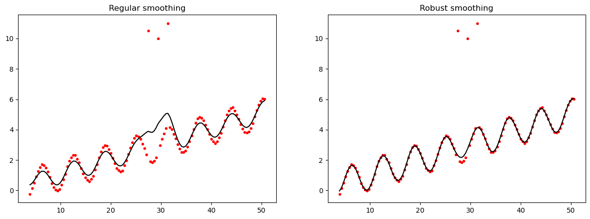
Example 1

1d array robust curve smoothing (with outliers)

x = np.linspace(0, 100, 2**8)
y = np.cos(x) + 0.1 * x + np.random.rand(2**8)*0.1
y[[70, 75, 80]] = [10.5, 10, 11]
y, x = y[10:130], x[10:130]

z_reg, s_reg, _, _ = smoothn(y.copy(), isrobust=False, debug_mode=False)  # Regular
z_rob, s_rob, _, _ = smoothn(y.copy(), isrobust=True, debug_mode=False)  # Robust

fig, axs = plt.subplots(1, 2, figsize=(15,5))
axs[0].plot(x, y, color='red', marker='.', linewidth=0)
axs[0].plot(x, z_reg, color='black')
axs[0].set_title("Regular smoothing")

axs[1].plot(x, y, color='red', marker='.', linewidth=0)
axs[1].plot(x, z_rob, color='black')
axs[1].set_title('Robust smoothing')
plt.show()

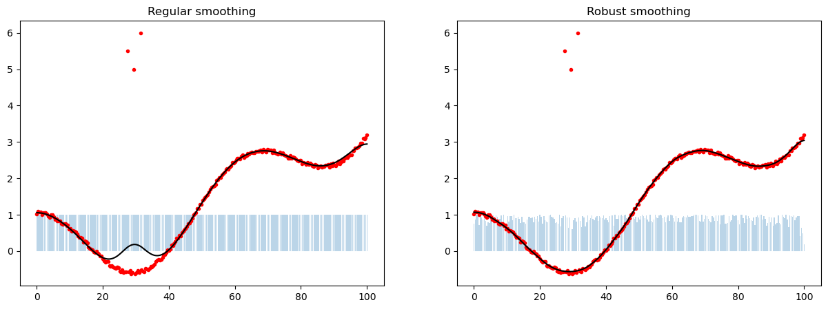
Example 2

1d array robust curve smoothing (with outliers) and updated weights

x = np.linspace(0, 100, 2 ** 8)
y = np.cos(x / 10) + (x / 50) ** 2 + np.random.rand(len(x)) / 10
y[[70, 75, 80]] = [5.5, 5, 6]

z_init_guess, dist = calc_init_guess(y, mask=np.isnan(y), coeff=0.1)
z_rob, s_rob, _, stats_rob = smoothn(
    y.copy(), isrobust=True, debug_mode=False, init_guess=z_init_guess,
    return_stats=('final_weights',))   # Robust
z_reg, s_reg, _, stats_reg = smoothn(
    y.copy(), isrobust=False, init_guess=z_init_guess,
    return_stats=('final_weights',))  # Regular

fig, axs = plt.subplots(1, 2, figsize=(15,5))
axs[0].plot(x, y, color='red', marker='.', linewidth=0)
axs[0].plot(x, z_reg, color='black')
axs[0].set_title("Regular smoothing")
axs[0].bar(x, stats_reg['final_weights'], alpha=0.3, width=0.3)

axs[1].plot(x, y, color='red', marker='.', linewidth=0)
axs[1].plot(x, z_rob, color='black')
axs[1].set_title('Robust smoothing')
axs[1].bar(x, stats_rob['final_weights'], alpha=0.3, width=0.3)

<BarContainer object of 256 artists>

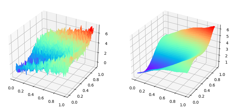
Example 3

Smoothing a surface

xp = np.arange(0, 1, 0.02)
[x,y] = np.meshgrid(xp, xp)
f = np.exp(x+y) + np.sin((x-2*y)*3)
fn = f + np.random.normal(size=f.size).reshape(f.shape) * 0.5
zr, smoothr, exit_flagr, statsr = smoothn(fn.copy())

fig, axs = plt.subplots(1, 2, subplot_kw={"projection": "3d"},
                       figsize=(10,5))
axs[0].plot_surface(x, y, fn, cmap=plt.get_cmap('rainbow'),
                    linewidth=2, antialiased=False)
axs[1].plot_surface(x, y, zr, cmap=plt.get_cmap('rainbow'),
                    linewidth=2, antialiased=False)

<mpl_toolkits.mplot3d.art3d.Poly3DCollection at 0x7f066d7e85f0>

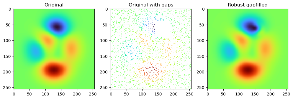
Example 4

Smooth 2d data with random and systematic gaps

n = 256
mat = loadmat(os.path.join(rootdir(), 'docs', 'examples', 'assets', '2d_peaks_n256.mat'))
y_original = mat['y0']
assert y_original.shape == (n, n)
idx = np.random.permutation(n**2)
y = y_original.flatten()
y[idx[:int(len(idx)/ 1.1)]] = np.nan
y = y.reshape(n,n)
y[40:90, 140:190] = np.nan
z_init_guess, dist = calc_init_guess(y.copy(), mask=np.isnan(y), coeff=0.1)
zr, smoothr, exitflagsr, statsr = smoothn(
    y.copy(), isrobust=True, gap_value=np.nan,
    init_guess=z_init_guess, debug_mode=False)   # Robust smoothing

z_init_guess_matlab = loadmat(os.path.join(rootdir(), 'docs', 'examples', 'assets', 'matlab_initguess.mat'))['z'][0][0]
zr_matlab, smoothr, exitflagsr, statsr = smoothn(
    y.copy(), isrobust=True, init_guess=z_init_guess_matlab,
    debug_mode=False)   # Robust smoothing

cmap = plt.get_cmap("turbo")
fig, axs = plt.subplots(1, 3, figsize=(12, 5))
axs[0].imshow(y_original, interpolation='none', cmap=cmap)
axs[0].set_title('Original')

axs[1].imshow(y, interpolation='none', cmap=cmap)
axs[1].set_title('Original with gaps')

axs[2].imshow(zr, interpolation='none', cmap=cmap)
axs[2].set_title('Robust gapfilled')

Text(0.5, 1.0, 'Robust gapfilled')

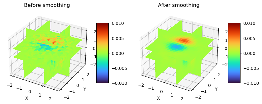
Example 5

Smoothing 3d array (volumetric) data

def plot_slices(x, y, z, data, xslices, yslices, zslices, ax, clim=(0,1)):
    data_n = data
    data_x = data_n[xslices,:,:]
    data_y = data_n[:,yslices,:]
    data_z = data_n[:,:,zslices]
    # Pick color map
    cmap = plt.get_cmap("turbo")
    norm = colors.Normalize(vmin=clim[0], vmax=clim[1])
    # Plot X slice
    data = {'x': [], 'y': [], 'z': []}
    for i, xslice in enumerate(xslices):
        d = data_x[i,:,:]
        data['x'].append(d)
        _ = ax.plot_surface(xslice, y[:, np.newaxis], z[np.newaxis, :],
                            rstride=1, cstride=1,
                            facecolors=cmap(norm(d)),
                            linewidth=3, antialiased=False,
                            shade=False)
    # Plot Y slice
    for i, yslice in enumerate(yslices):
        d = data_y[:,i,:]
        data['y'].append(d)
        _ = ax.plot_surface(x[:, np.newaxis], yslice, z[np.newaxis, :],
                            rstride=1, cstride=1,
                            facecolors=cmap(norm(d)),
                            linewidth=1, antialiased=False,
                            shade=False)
    # Plot Z slice
    for i, zslice in enumerate(zslices):
        d = data_z[:,:,i]
        data['z'].append(d)
        _ = ax.plot_surface(x[:, np.newaxis], y[np.newaxis, :],
                            np.atleast_2d(zslice),
                            rstride=1, cstride=1,
                            facecolors=cmap(norm(d)),
                            linewidth=1, antialiased=False,
                            shade=False)

    ax.set_xlabel('X')
    ax.set_ylabel('Y')
    ax.set_zlabel('Z')

    sl = cm.ScalarMappable(cmap=cmap, norm=norm)
    sl.set_array([])

    return sl, data


x = np.linspace(-2, 2.2, 21)
y = np.linspace(-2, 2.2, 19)
z = np.linspace(-2, 2.2, 17)
_x, _y, _z = np.meshgrid(y,x,z)
vn = _x * np.exp(-_x**2-_y**2-_z**2) + \
     (np.reshape(np.random.normal(size=_x.shape) * 0.01, _x.shape))

offset = np.outer(np.outer(slide(stop=1.1), slide(stop=1.0)),
                  slide(stop=0.9)).reshape(21,19,17)
vn *= offset

clim = (-0.01, 0.01)
xslices = np.array([-1, 1])
yslices = np.array([0])
zslices = np.array([0, 1])

fig, axs = plt.subplots(1, 2, figsize=(10,5), subplot_kw=dict(projection='3d'))
im, data = plot_slices(x, y, z, vn,
            xslices, yslices, zslices,
            axs[0], clim=clim)
fig.colorbar(im, shrink=0.5, aspect=5, ax=axs[0])
axs[0].set_title('Before smoothing')

v, smooth, flags, stats = smoothn(vn.copy(), isrobust=True)
im, data = plot_slices(x, y, z, v,
            xslices, yslices, zslices,
            axs[1], clim=(-0.01, 0.01))
fig.colorbar(im, shrink=0.5, aspect=5, ax=axs[1])
axs[1].set_title('After smoothing')

Text(0.5, 0.92, 'After smoothing')

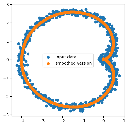
Example 6

Smoothing a cardioid

t = np.linspace(0, 2*np.pi, 1000)
x = 2*np.cos(t)*(1-np.cos(t)) + np.random.normal(size=t.size).reshape(t.shape)*0.1
y = 2*np.sin(t)*(1-np.cos(t)) + np.random.normal(size=t.size).reshape(t.shape)*0.1
x[123], y[524] = -9999, -9999 # add a few fill values to test if they are ignored correctly
z, smooth, flags, stats = smoothn(np.array([x, y]).copy(), axis=(1,))
x[123], y[524] = np.nan, np.nan
fig, ax = plt.subplots(1,1, figsize=(5, 5))
ax.scatter(x, y, label='input data')
ax.scatter(*z, label='smoothed fit')
plt.legend()

<matplotlib.legend.Legend at 0x7f066caa0e00>

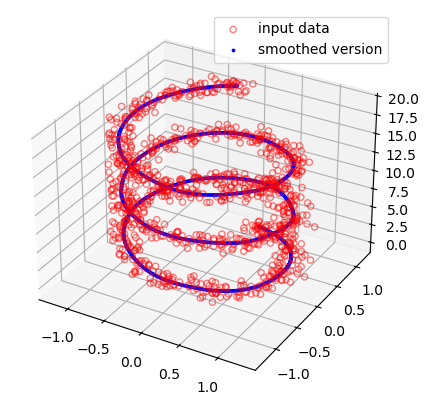
Example 7

Smoothing a 3d parametric curve

t = np.linspace(0, 6*np.pi, 1000)
x = np.sin(t) + np.random.normal(size=t.size).reshape(t.shape)*0.1
y = np.cos(t) + np.random.normal(size=t.size).reshape(t.shape)*0.1
z = t +  np.random.normal(size=t.size).reshape(t.shape)*0.1
u, smooth, flags, stats = smoothn(np.array([x,y,z]).copy(), axis=(1,))

fig = plt.figure(figsize=(5,5))
ax = fig.add_subplot(1,1,1, projection='3d')
ax.scatter(x,y,z, facecolors='none', edgecolors='red', alpha=0.5, label='input data')
ax.scatter(*u, facecolors='blue', edgecolors='blue', alpha=1, s=3, label='smoothed fit')
plt.legend()

<matplotlib.legend.Legend at 0x7f066d0ac5c0>

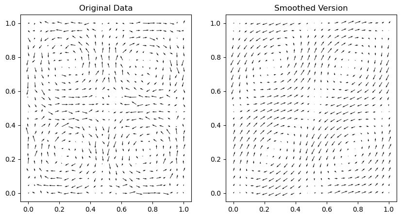
Example 8

Smoothing a 2d vector field

t = np.linspace(0, 1, 24)
[x,y] = np.meshgrid(t,t)
Vx = np.cos(2*np.pi*x+np.pi/2)*np.cos(2*np.pi*y)
Vy = np.sin(2*np.pi*x+np.pi/2)*np.sin(2*np.pi*y)
# Add Noise
Vx = Vx + np.sqrt(0.05)*np.random.normal(size=x.size).reshape(x.shape)
Vy = Vy + np.sqrt(0.05)*np.random.normal(size=x.size).reshape(x.shape)
I = np.random.permutation(Vx.size)
# Add Outliers
Vx.flatten()[I[:30]] = (np.random.normal(size=30)-0.5) * 5
Vx = Vx.reshape(Vy.shape)
Vy.flatten()[I[:30]] = (np.random.normal(size=30)-0.5) * 5
Vy = Vy.reshape(Vx.shape)
# Missing values
Vy.flatten()[I[30:60]] = np.nan
Vy = Vy.reshape(Vx.shape)
Vx.flatten()[I[30:60]] = np.nan
Vx = Vx.reshape(Vy.shape)
Vs, smooth, flags, stats = smoothn(np.array([Vx, Vy]).copy(), isrobust=True)

fig, axs = plt.subplots(1, 2, figsize=(10,5))
axs[0].quiver(x, y, Vx, Vy)
axs[0].set_title("Original Data")
axs[1].quiver(x, y, *Vs)
axs[1].set_title("Smoothed Version")

Text(0.5, 1.0, 'Smoothed Version')

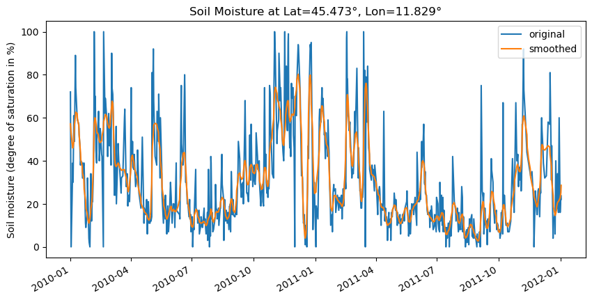
Example 9 - Smoothing a soil moisture time series (1d)

Here we apply the DCT-PLS algorithm to a 1d soil moisture time series from HSAF ASCAT. Note that in practice it is recommended to also use the spatial neigbourhood information to smooth or interpolate soil moisture, not only the temporal one, as done in this example.

import warnings
from ascat.read_native.cdr import AscatGriddedNcTs
import pandas as pd

testdata_path = rootdir() / "tests" / "test-data"
ascat_data_folder = testdata_path / "sat" / "ascat" / "netcdf" / "55R22"
ascat_grid_fname = testdata_path / "sat" / "ascat" / "netcdf" / "grid" / "TUW_WARP5_grid_info_2_1.nc"
static_layer_path = testdata_path / "sat" / "h_saf" / "static_layer"


#init the AscatSsmCdr reader with the paths
with warnings.catch_warnings():
    warnings.filterwarnings('ignore') # some warnings are expected and ignored

    ascat_reader = AscatGriddedNcTs(
        ascat_data_folder,
        "TUW_METOP_ASCAT_WARP55R22_{:04d}",
        grid_filename=ascat_grid_fname,
        static_layer_path=static_layer_path
    )

lat, lon = 45.473, 11.829
ascat_ts = ascat_reader.read(lon, lat)['sm']
data, _, _, _= smoothn(ascat_ts.values, isrobust=True)
ascat_ts_smoothed = pd.Series(data, ascat_ts.index.values)
fig, ax = plt.subplots(1, 1, figsize=(10,5))
ascat_ts.loc['2010-01-01':'2012-01-01'].plot(label='original', ax=ax)
ascat_ts_smoothed.loc['2010-01-01':'2012-01-01'].plot(label='smoothed', ax=ax)
plt.title(f"Soil Moisture at Lat={lat}°, Lon={lon}°")
plt.ylabel("Soil moisture (degree of saturation in %)")
plt.legend()

<matplotlib.legend.Legend at 0x7f066cfa2810>